amitlad.com - Horror Movies

Introduction

This week’s data set is contains information about Horror Movies dating back to the 1950s. The data was extracted from the Movie Database.

Hypostheses

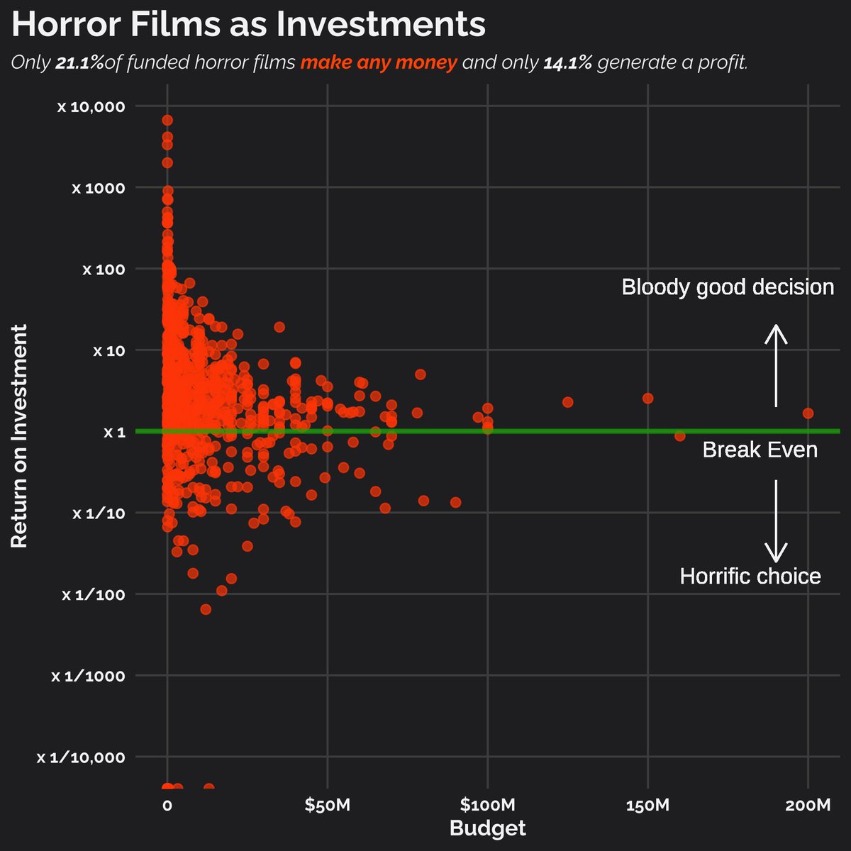
Prior to starting, I saw that @zakvarty had produced a visualisation showing that horror movies are probably not a good investment:

I wanted to see if it was possible to find a good horror movie investment strategy…

Findings

Show the code

library(tidyverse)
library(tidytuesdayR)
library(here)
library(lubridate)

tt_data <- read_rds(paste0(here("posts","TT_2022_wk44_HorrorMovies"), "/tt_data.rds"))
horror_movies <- tt_data$horror_movies

It turns out there is huge volatility in the returns on investment. There is no easy to identify traits for films to guarantee big profits.

However, the industry as a whole delivers strong positive returns year after year, even after the start of the Covid-19 pandemic. If you can find a passive index tracker that invests in Horror Movies, then you might want to consider adding it to your asset allocation… [This is not serious investment advice!]

Show the code

# Wrangle data -----------------------------------------------------------------
horror_movies_returns <-
  horror_movies %>%
  mutate(
    release_month = month(release_date), 
    release_year = year(release_date),
    gross_return = revenue / budget, 
    gross_return_all = sum(revenue) / sum(budget)
    ) %>%
  group_by(release_year) %>%
  mutate(
    gross_return_YYYY = sum(revenue) / sum(budget), 
    total_budget_YYYY = sum(budget),
    number_of_films_YYYY = n()
    ) %>%
  ungroup() %>%
  group_by(release_month) %>%
  mutate(
    gross_return_MM = sum(revenue) / sum(budget), 
    total_budget_MM = sum(budget),
    number_of_films_MM = n()
    ) %>%
  ungroup() %>%
  group_by(release_year, release_month) %>%
  mutate(
    gross_return_YYYY_MM = sum(revenue) / sum(budget), 
    total_budget_YYYY_MM = sum(budget),
    number_of_films_YYYY_MM = n()
    ) %>%
  ungroup()

# Plotting preparation ---------------------------------------------------------

# Title
title_text <- "In aggregate, horror movies have delivered a strong return on investment"
subtitle_text <- "
    Return on investment calculated as (Revenue / Budget), costs above budget not considered.
    Small points show individual Horror films.  Large points show films grouped by release year.
    Size of large points reflects number of films released that year."
caption_text <- "#TidyTuesday 2022 wk44 | Data: The Movie Database | Viz: Amit Lad | Inspired by @zakvarty"

# Axis
x_breaks <- NULL
x_labels <- NULL
x_limits <- c(as_date("1995-01-01"), as_date("2022-12-31"))
x_title <- "Release date"

y_breaks <- c(1e-2, 1e-1, 1e0, 1e1, 1e2, 1e3)
y_labels <- c("x 1/100", "x 1/10", "x 1", "x 10", "x 100", "x 1000")
y_limits <- c(1e-1, 2e1)
y_title <- "Return on investment"

## Plot colour palette
bg_colour <- "#28282B"
text_colour <- "#F5F5F5"
annotation_colour <- "#85E21F"

# Buid plot -------------------------------------------------------------------

ggplot(
  data = horror_movies_returns, 
  mapping = aes(x = as_date(paste0(release_year,"0630")), y = gross_return_YYYY)) +
  geom_point(aes(x = release_date, y = gross_return, alpha = 0, size = 0), show.legend = FALSE) +
  geom_point(aes(size = number_of_films_YYYY, colour = "#F75F1C"), show.legend = FALSE) +
  geom_hline(yintercept = 1, colour = "#881EE4") +
  geom_vline(xintercept = as_date("2020-03-19"), colour = "#881EE4") +
  scale_y_log10(
    breaks = y_breaks,
    labels = y_labels,
    limits = y_limits,
    ) +
  xlim(x_limits) +
  annotate(
    geom = "text",
    x = as_date("1993-12-3"),
    y = 0.8,
    label = "Revenue = budget",
    colour = "#881EE4"
  ) +
  annotate(
    geom = "text",
    x = as_date("2020-11-30"),
    y = 0.3,
    label = "Covid-19",
    colour = "#881EE4",
    angle = 90
  ) +
  annotate(
    geom = "text",
    x = as_date("2005-6-30"),
    y = 0.3,
    label = "Large volatility in returns for individual films.
    Strong positive return at aggregate level each year, even after Covid-19.",
    colour = annotation_colour
  ) +
  labs(title = title_text, subtitle = subtitle_text, caption = caption_text, x = x_title, y = y_title) +
  theme(
    text = element_text(face = "bold", colour = text_colour),
    plot.title.position = "plot",
    plot.caption.position = "plot",
    # plot.title = element_text(hjust = 0, size = 18),
    # plot.subtitle = element_markdown(size = 10, face = "italic"),
    axis.text = element_text(colour = text_colour),
    panel.grid.minor = element_line(colour = "grey10"),
    panel.grid.major = element_line(colour = "grey30"),
    plot.background = element_rect(fill = bg_colour, colour = bg_colour),
    panel.background = element_rect(fill = bg_colour, colour = bg_colour))

Looking at sub-genre, pure Horror movies are the best, closely followed by Horror-Thrillers. I’d stay away from investing in Horror Histories, Horror Musicals, Horror Documentaries and Horror Westerns!

Show the code

# Wrangle data -----------------------------------------------------------------
horror_movies_returns_genre <-
  horror_movies_returns %>%
  separate_rows(genre_names) %>%
  filter(genre_names != "Horror") %>%
  bind_rows(filter(horror_movies_returns, genre_names == "Horror")) %>%
  group_by(genre_names) %>%
  summarise(
    gross_return_genre = sum(revenue) / sum(budget), 
    total_budget_genre = sum(budget),
    number_of_films_genre = n(),
    gross_return_all = mean(gross_return_all)
    ) %>%
  ungroup() %>%
  arrange(gross_return_genre, increasing = TRUE) %>% 
  filter(genre_names != "TV", genre_names != "Movie") %>%
  mutate(rank = rank(gross_return_genre, ties.method = "first"))


# Plotting preparation ---------------------------------------------------------

# Title
title_text <- "Return on investment (for all time) for Horror Movie subgenres."
subtitle_text <- "
    Return on investment calculated as (Revenue / Budget), costs above budget not considered.
    \"Horror\" category means no sub-genre."
caption_text <- "#TidyTuesday 2022 wk44 | Data: The Movie Database | Viz: Amit Lad | Inspired by @zakvarty"

# Axis
y_breaks <- c(1:19)
y_labels <- horror_movies_returns_genre$genre_names
y_limits <- NULL
y_title <- "Genre"

x_breaks <- c(1e-2, 1e-1, 1e0, 1e1, 1e2, 1e3)
x_labels <- c("x 1/100", "x 1/10", "x 1", "x 10", "x 100", "x 1000")
x_limits <- c(0.5e-1, 2.5)
x_title <- "Return on investment"

# Plot colour palette
bg_colour <- "#28282B"
text_colour <- "#F5F5F5"
annotation_colour <- "#85E21F"

# Build plot -------------------------------------------------------------------

ggplot(
  data = horror_movies_returns_genre, 
  mapping = aes()
  ) +
  geom_segment(
    aes(
      x = gross_return_genre, 
      xend = 1,
      y = rank,
      yend = rank, 
      colour = as.factor(rank)
      ), 
    size = 3,
    show.legend = FALSE) +
  geom_vline(xintercept = 1, colour = "#881EE4") +
    scale_y_continuous(
    name = NULL,
    breaks = y_breaks,
    labels = y_labels
    ) +
  scale_x_continuous(
    name = "Return on investment (= Revenue / Budget)",
    breaks = c(0, 0.5, 1, 1.5, 2, 2.5, 3),
    labels = c("0.0x", "0.5x", "1.0x", "1.5x", "2.0x", "2.5%", "3.0x"),
    limits = c(0,3),
    ) +
  labs(title = title_text, subtitle = subtitle_text, caption = caption_text, x = x_title, y = y_title) +
  theme(
    text = element_text(face = "bold", colour = text_colour),
    plot.title.position = "plot",
    plot.caption.position = "plot",
    # plot.title = element_text(hjust = 0, size = 18),
    # plot.subtitle = element_markdown(size = 10, face = "italic"),
    axis.text = element_text(colour = text_colour),
    panel.grid.minor = element_line(colour = "grey10"),
    panel.grid.major = element_line(colour = "grey30"),
    plot.background = element_rect(fill = bg_colour, colour = bg_colour),
    panel.background = element_rect(fill = bg_colour, colour = bg_colour))

Showcase of other people’s visualisations work

@PauBaudry

@cararthompson

@cyd_yzc

@jim_gruman

@nicci_potts

Citation

BibTeX citation:

@online{lad2022,
  author = {Amit Lad},
  title = {Horror {Movies}},
  date = {2022-11-05},
  url = {https://amitlad.com/posts/TT_2022_wk44_HorrorMovies/post.html},
  langid = {en}
}

For attribution, please cite this work as:

Amit Lad. 2022. “Horror Movies.” November 5, 2022. https://amitlad.com/posts/TT_2022_wk44_HorrorMovies/post.html.

--- title: 'Horror Movies' date: '2022-11-05' categories: ['TidyTuesday', 'RStats'] description: 'TidyTuesday 2022wk44' execute: message: false warning: false format: html: code-fold: true code-summary: "Show the code" code-tools: true editor_options: chunk_output_type: console draft: false image: tt_Horror_amitlad.png --- ### Introduction This week's data set is contains information about Horror Movies dating back to the 1950s. The data was extracted from the [Movie Database](https://www.themoviedb.org). ### Hypostheses Prior to starting, I saw that @zakvarty had produced a visualisation showing that horror movies are probably not a good investment: [![](tt_Horror_01.jpeg)](https://twitter.com/zakvarty/status/1587798613106823168?s=20&t=1aqQl06dvtrTwO4pTjxbAQ) I wanted to see if it was possible to find a good horror movie investment strategy... ### Findings ```{r download_data} library(tidyverse) library(tidytuesdayR) library(here) library(lubridate) tt_data <- read_rds(paste0(here("posts","TT_2022_wk44_HorrorMovies"), "/tt_data.rds")) horror_movies <- tt_data$horror_movies ``` It turns out there is huge volatility in the returns on investment. There is no easy to identify traits for films to guarantee big profits. However, the industry as a whole delivers strong positive returns year after year, even after the start of the Covid-19 pandemic. If you can find a passive index tracker that invests in Horror Movies, then you might want to consider adding it to your asset allocation... [This is not serious investment advice!] ```{r horror_movie_investment} # Wrangle data ----------------------------------------------------------------- horror_movies_returns <- horror_movies %>% mutate( release_month = month(release_date), release_year = year(release_date), gross_return = revenue / budget, gross_return_all = sum(revenue) / sum(budget) ) %>% group_by(release_year) %>% mutate( gross_return_YYYY = sum(revenue) / sum(budget), total_budget_YYYY = sum(budget), number_of_films_YYYY = n() ) %>% ungroup() %>% group_by(release_month) %>% mutate( gross_return_MM = sum(revenue) / sum(budget), total_budget_MM = sum(budget), number_of_films_MM = n() ) %>% ungroup() %>% group_by(release_year, release_month) %>% mutate( gross_return_YYYY_MM = sum(revenue) / sum(budget), total_budget_YYYY_MM = sum(budget), number_of_films_YYYY_MM = n() ) %>% ungroup() # Plotting preparation --------------------------------------------------------- # Title title_text <- "In aggregate, horror movies have delivered a strong return on investment" subtitle_text <- " Return on investment calculated as (Revenue / Budget), costs above budget not considered. Small points show individual Horror films. Large points show films grouped by release year. Size of large points reflects number of films released that year." caption_text <- "#TidyTuesday 2022 wk44 | Data: The Movie Database | Viz: Amit Lad | Inspired by @zakvarty" # Axis x_breaks <- NULL x_labels <- NULL x_limits <- c(as_date("1995-01-01"), as_date("2022-12-31")) x_title <- "Release date" y_breaks <- c(1e-2, 1e-1, 1e0, 1e1, 1e2, 1e3) y_labels <- c("x 1/100", "x 1/10", "x 1", "x 10", "x 100", "x 1000") y_limits <- c(1e-1, 2e1) y_title <- "Return on investment" ## Plot colour palette bg_colour <- "#28282B" text_colour <- "#F5F5F5" annotation_colour <- "#85E21F" # Buid plot ------------------------------------------------------------------- ggplot( data = horror_movies_returns, mapping = aes(x = as_date(paste0(release_year,"0630")), y = gross_return_YYYY)) + geom_point(aes(x = release_date, y = gross_return, alpha = 0, size = 0), show.legend = FALSE) + geom_point(aes(size = number_of_films_YYYY, colour = "#F75F1C"), show.legend = FALSE) + geom_hline(yintercept = 1, colour = "#881EE4") + geom_vline(xintercept = as_date("2020-03-19"), colour = "#881EE4") + scale_y_log10( breaks = y_breaks, labels = y_labels, limits = y_limits, ) + xlim(x_limits) + annotate( geom = "text", x = as_date("1993-12-3"), y = 0.8, label = "Revenue = budget", colour = "#881EE4" ) + annotate( geom = "text", x = as_date("2020-11-30"), y = 0.3, label = "Covid-19", colour = "#881EE4", angle = 90 ) + annotate( geom = "text", x = as_date("2005-6-30"), y = 0.3, label = "Large volatility in returns for individual films. Strong positive return at aggregate level each year, even after Covid-19.", colour = annotation_colour ) + labs(title = title_text, subtitle = subtitle_text, caption = caption_text, x = x_title, y = y_title) + theme( text = element_text(face = "bold", colour = text_colour), plot.title.position = "plot", plot.caption.position = "plot", # plot.title = element_text(hjust = 0, size = 18), # plot.subtitle = element_markdown(size = 10, face = "italic"), axis.text = element_text(colour = text_colour), panel.grid.minor = element_line(colour = "grey10"), panel.grid.major = element_line(colour = "grey30"), plot.background = element_rect(fill = bg_colour, colour = bg_colour), panel.background = element_rect(fill = bg_colour, colour = bg_colour)) ``` Looking at sub-genre, pure Horror movies are the best, closely followed by Horror-Thrillers. I'd stay away from investing in Horror Histories, Horror Musicals, Horror Documentaries and Horror Westerns! ```{r horror_movie_genre} # Wrangle data ----------------------------------------------------------------- horror_movies_returns_genre <- horror_movies_returns %>% separate_rows(genre_names) %>% filter(genre_names != "Horror") %>% bind_rows(filter(horror_movies_returns, genre_names == "Horror")) %>% group_by(genre_names) %>% summarise( gross_return_genre = sum(revenue) / sum(budget), total_budget_genre = sum(budget), number_of_films_genre = n(), gross_return_all = mean(gross_return_all) ) %>% ungroup() %>% arrange(gross_return_genre, increasing = TRUE) %>% filter(genre_names != "TV", genre_names != "Movie") %>% mutate(rank = rank(gross_return_genre, ties.method = "first")) # Plotting preparation --------------------------------------------------------- # Title title_text <- "Return on investment (for all time) for Horror Movie subgenres." subtitle_text <- " Return on investment calculated as (Revenue / Budget), costs above budget not considered. \"Horror\" category means no sub-genre." caption_text <- "#TidyTuesday 2022 wk44 | Data: The Movie Database | Viz: Amit Lad | Inspired by @zakvarty" # Axis y_breaks <- c(1:19) y_labels <- horror_movies_returns_genre$genre_names y_limits <- NULL y_title <- "Genre" x_breaks <- c(1e-2, 1e-1, 1e0, 1e1, 1e2, 1e3) x_labels <- c("x 1/100", "x 1/10", "x 1", "x 10", "x 100", "x 1000") x_limits <- c(0.5e-1, 2.5) x_title <- "Return on investment" # Plot colour palette bg_colour <- "#28282B" text_colour <- "#F5F5F5" annotation_colour <- "#85E21F" # Build plot ------------------------------------------------------------------- ggplot( data = horror_movies_returns_genre, mapping = aes() ) + geom_segment( aes( x = gross_return_genre, xend = 1, y = rank, yend = rank, colour = as.factor(rank) ), size = 3, show.legend = FALSE) + geom_vline(xintercept = 1, colour = "#881EE4") + scale_y_continuous( name = NULL, breaks = y_breaks, labels = y_labels ) + scale_x_continuous( name = "Return on investment (= Revenue / Budget)", breaks = c(0, 0.5, 1, 1.5, 2, 2.5, 3), labels = c("0.0x", "0.5x", "1.0x", "1.5x", "2.0x", "2.5%", "3.0x"), limits = c(0,3), ) + labs(title = title_text, subtitle = subtitle_text, caption = caption_text, x = x_title, y = y_title) + theme( text = element_text(face = "bold", colour = text_colour), plot.title.position = "plot", plot.caption.position = "plot", # plot.title = element_text(hjust = 0, size = 18), # plot.subtitle = element_markdown(size = 10, face = "italic"), axis.text = element_text(colour = text_colour), panel.grid.minor = element_line(colour = "grey10"), panel.grid.major = element_line(colour = "grey30"), plot.background = element_rect(fill = bg_colour, colour = bg_colour), panel.background = element_rect(fill = bg_colour, colour = bg_colour)) ``` ### Showcase of other people's visualisations work #### @PauBaudry [![\@PauBaudry](tt_Horror_03.jpeg)](https://twitter.com/PauBaudry/status/1588228496957919232) #### @cararthompson [![\@amycjack](tt_Horror_02.jpeg)](https://twitter.com/amycjack/status/1588512418094669825) #### @cyd_yzc [![\@cyd_yzc](tt_Horror_04.jpeg)](https://twitter.com/Cyd_yzc/status/1588154144623304705) #### @jim_gruman [![\@jim_gruman](tt_Horror_05.jpeg)](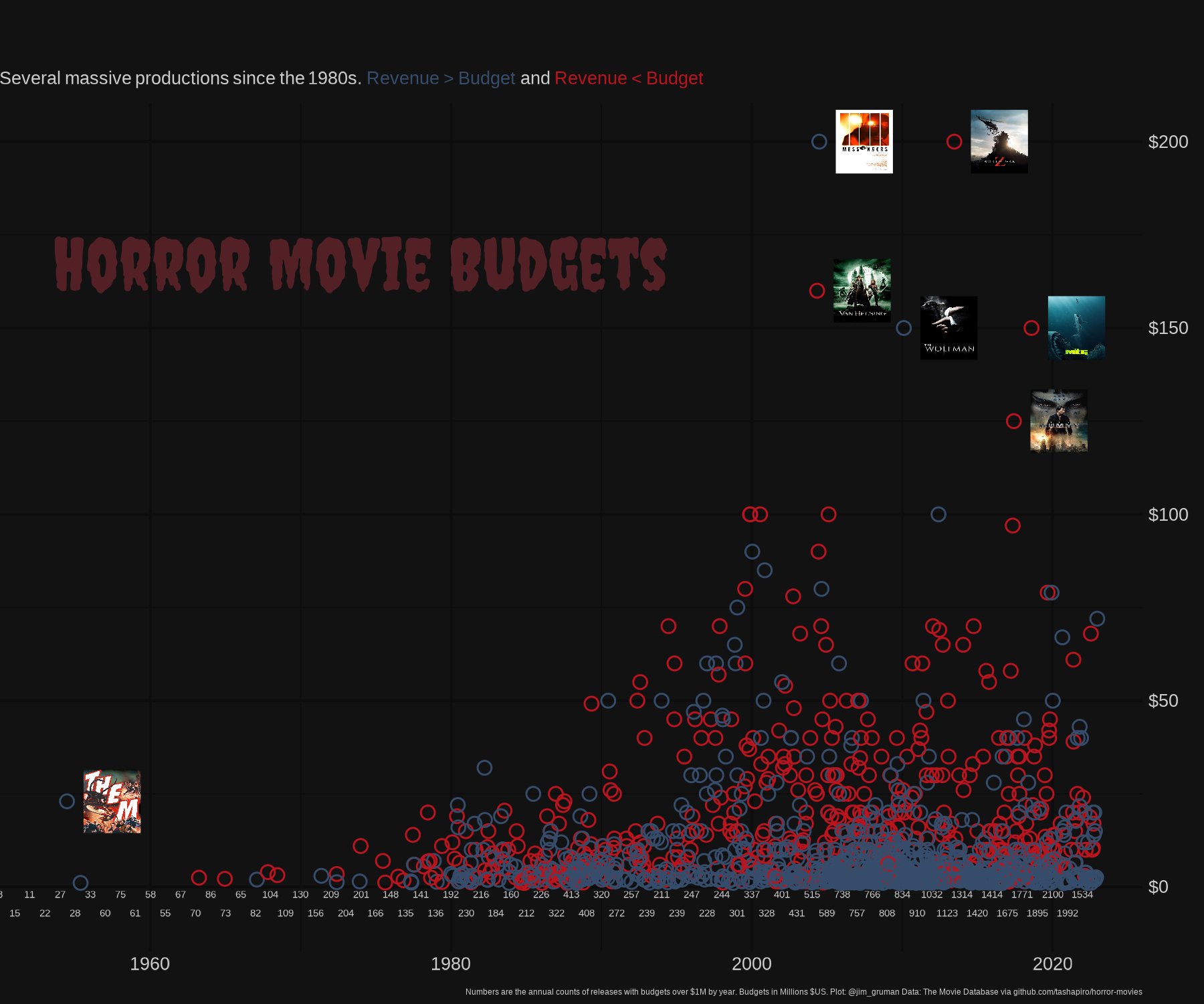https://twitter.com/jim_gruman/status/1587942905951420422) #### @nicci_potts [![\@nicci_potts](tt_Horror_06.png)](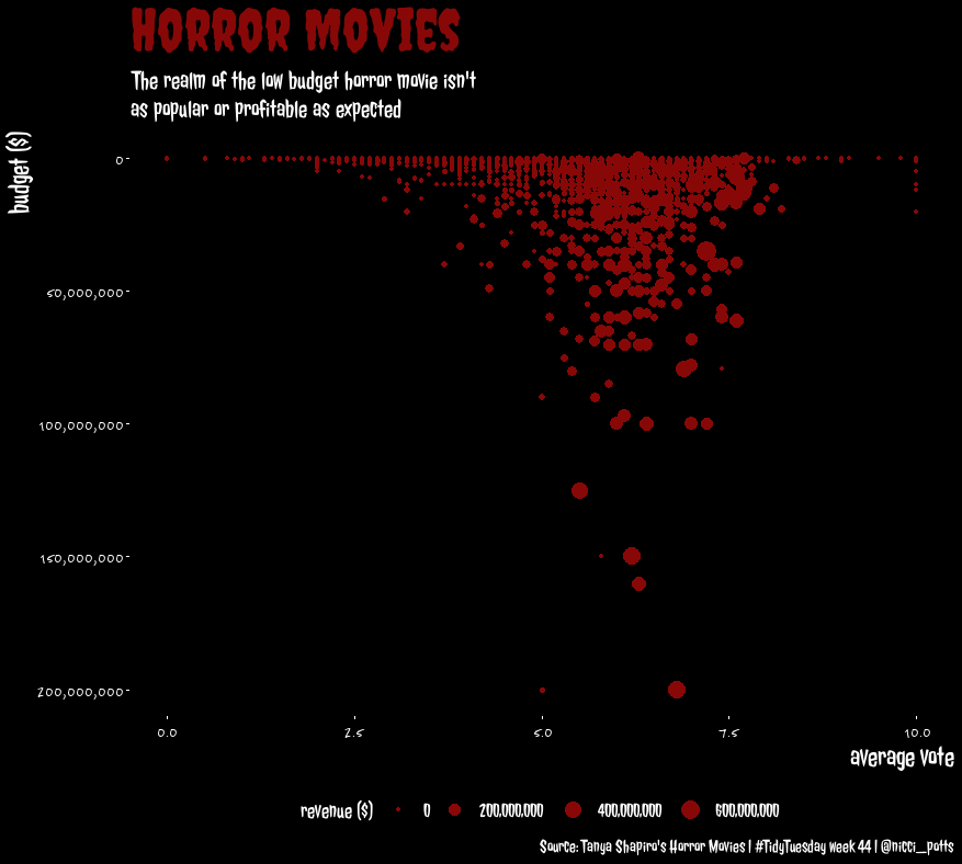https://twitter.com/nicci_potts/status/1587878659125280771?s=20&t=1aqQl06dvtrTwO4pTjxbAQ)